Understanding Postgres EXPLAIN Output
介绍 #
🌐 Introduction
本指南旨在帮助你了解如何使用 Postgres 的 EXPLAIN 和 EXPLAIN ANALYZE 命令来优化和调试 SQL 查询。理解这些命令的输出可以帮助你通过优化数据库交互来提升应用的性能。
🌐 This guide is designed to help you understand how to use the Postgres EXPLAIN and EXPLAIN ANALYZE commands to optimize and debug SQL queries. Understanding the output of these commands can help you improve the performance of your applications by optimizing database interactions.
解释是什么? #
🌐 What is explain?
Postgres 的 EXPLAIN 命令会显示 SQL 查询的执行计划。这个计划会说明 Postgres 数据库将如何执行查询,包括如何扫描表——比如使用顺序扫描、索引扫描等——以及如何将行进行连接。
🌐 The Postgres EXPLAIN command shows the execution plan of a SQL query. This plan describes how the Postgres database will execute the query, including how tables will be scanned—by using sequential scans, index scans, etc.—and how rows will be joined.
如何在 Supabase 中使用 explain #
🌐 How to use explain in Supabase
通过 SQL 编辑器使用 EXPLAIN
- 访问你的 Supabase 项目
- 打开 SQL 编辑器
- 用你的查询执行 EXPLAIN:
EXPLAIN SELECT * FROM users WHERE user_id = 1;
在 supabase-js 库中使用 EXPLAIN
1const { data, error } = await supabase2 .from('countries')3 .select()4 .explain({analyze:true,verbose:true})解释输出组件的详细拆解 #
🌐 Detailed breakdown of explain output components
1. 计划类型 #
🌐 1. Plan type
- 顺序扫描: 一种顺序扫描,会读取表中的所有行。通常在查询没有可用索引时会看到这种情况。
- 索引扫描: 使用索引高效地查找行。这表示查询能够使用索引来高效定位数据。
- 位图堆扫描: 使用位图索引有效地查找行,然后从表中检索实际行。当需要检索适量行时,这种扫描方式很高效。
2. 成本 #
🌐 2. Cost
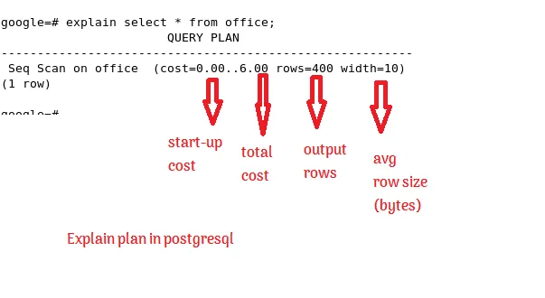
cost=0.00..19.00: 这表示执行该计划的预计成本。第一个数字 (0.00) 是返回第一行的成本,第二个数字 (19.00) 是执行查询并获取所有行的总成本。这些值是数据库成本模型确定的任意单位,而不是实际的时间或资源。
启动成本: 在返回第一行之前产生的成本。 总成本: 操作的预计总成本。
3. 行 #
🌐 3. Rows
rows=1: 这是查询将返回的行数的估计值。准确的行数估计依赖于最新的统计信息;如果估计不准确,可能意味着数据库的统计信息需要更新。
4. 宽度 #
🌐 4. Width
width=240: 输出行预计的平均字节数。这表明需要处理或传输的预期数据量,可能会影响性能。
5. 过滤器 #
🌐 5. Filters
过滤器: (user_id = 1): 这显示扫描后应用的任何过滤器。过滤器是在检索行之后检查的条件。如果被过滤掉的行数很多,可能意味着需要更好的索引。
6. 执行时间 #
🌐 6. Execution time
执行时间: 0.069 毫秒: 测量执行查询所花的时间,包括检索数据、执行任何排序、连接或执行计划中定义的其他操作,以及返回最终结果。这个时间以毫秒为单位。
详细组件在解释分析中 #
🌐 Detailed components in explain analyze
运行 EXPLAIN ANALYZE 时,会提供额外的信息,包括:
🌐 When running EXPLAIN ANALYZE, additional information is provided, including:
- 实际时间: 显示执行扫描和获取行所花费的时间。它分为获取第一行所花费的时间(first)和获取所有行所花费的时间(last)。
- 被过滤删除的行数: 表示有多少行因不符合过滤条件而被排除。
- 循环: 显示节点执行了多少次,尤其是在嵌套循环连接或子查询中相关。
详细 EXPLAIN ANALYZE 输出示例
🌐 Example of Detailed EXPLAIN ANALYZE Output
1Seq Scan on users (cost=0.00..19.00 rows=1 width=240) (actual time=0.026..0.026 rows=1 loops=1)2 Filter: (user_id = 1)3 Rows Removed by Filter: 9994Planning Time: 0.135 ms- 实际时间=0.026..0.026: 开始返回行到全部返回完成所用的时间。
- 被过滤器移除的行: 999:表示很多行已经被过滤器检查过,但大多数不符合条件。
- 规划时间:0.135 毫秒: 规划时间指的是 Postgres 查询规划器分析查询并创建执行计划所花费的时间。这个时间以毫秒为单位测量。
你现在可能会问自己,为什么会有两套不同的指标:(cost=0.42..2.64 rows=1 width=164) (actual time=0.020..0.021 rows=1 loops=1)#
🌐 You might be asking yourself now, why there is two different sets of metrics : (cost=0.42..2.64 rows=1 width=164) (actual time=0.020..0.021 rows=1 loops=1)?
回答你,上面解释过的,一个是用于估算成本和性能的,另一个是用于查询的实际性能的。
🌐 To answer you, one is for the estimated cost and performance, and another for the actual performance of the query as explained above.
计划 vs. 执行:这些估算是基于查询优化器对数据的理解(通过表的大小、值的分布等统计信息收集),而实际指标则告诉你查询运行时真正发生了什么。这个对比可以揭示优化器假设中的不准确之处。
性能调优:通过比较估计行数和实际行数,或者估计时间和实际时间,你可以发现潜在的性能问题。例如,如果估计行数与实际行数差距很大,可能说明表的统计信息已经过时,从而导致查询计划效率低下。
识别瓶颈:如果实际耗时明显高于预期,或者循环比预计更频繁,这些都可能是查询性能瓶颈的信号。
如何阅读复杂的 explain 输出 #
🌐 How to read a complex explain output
首先,你得明白,Postgres 的执行计划是一个由多个节点组成的树状结构。最顶上的节点(上面的 Aggregate)在最上面,下面的节点缩进显示,并以箭头(->)开头。缩进相同的节点表示处于同一层级(比如用 join 结合的两个关系)。
🌐 First, you have to understand that a Postgres execution plan is a tree structure consisting of several nodes. The top node (the Aggregate above) is at the top, and lower nodes are indented and start with an arrow (->). Nodes with the same indentation are on the same level (for example, the two relations combined with a join).
这里有一个例子:
🌐 Here's an example:
1Aggregate Node (Top Node)2│3└──> Sort Node4 │5 └──> Hash Join Node6 │7 ├──> Seq Scan on users (Filtered)8 │9 └──> Hash10 │11 └──> Seq Scan on activitiesPostgres 是自上而下执行计划的,也就是说,它从生成顶层节点的第一行结果开始。执行器按“需要”处理下层节点,也就是说,它只会从下层节点获取计算上层节点下一个结果所需的行数。这会影响你如何理解“成本”和“时间”:上层节点的启动时间至少跟下层节点的启动时间一样高,总时间也是如此。如果你想知道某个节点实际花费的时间,就必须减去下层节点花费的时间。并行查询会让这个情况更复杂。
🌐 Postgres executes a plan top down, that is, it starts with producing the first result row for the top node. The executor processes lower nodes “on demand”, that is, it fetches only as many result rows from them as it needs to calculate the next result of the upper node. This influences how you have to read “cost” and “time”: the startup time for the upper node is at least as high as the startup time of the lower nodes, and the same holds for the total time. If you want to find the net time spent in a node, you have to subtract the time spent in the lower nodes. Parallel queries make that even more complicated.
除此之外,你还得用“循环”的次数乘以成本和时间,才能算出在一个节点上花的总时间。
🌐 On top of that, you have to multiply the cost and the time with the number of “loops” to get the total time spent in a node.
Postgres 执行计划输出中的常见节点 #
🌐 Common nodes in Postgres explain output
| 节点类型 | 描述 |
|---|---|
| 序列扫描 | 顺序扫描表中的每一行,通常在没有合适索引时使用。 |
| 索引扫描 | 使用索引高效查找行,对于小部分行非常高效。 |
| 仅索引扫描 | 直接从索引获取所需的所有数据,无需访问表。 |
| 位图堆扫描 | 使用行位置的位图来高效地从表中获取行。 |
| 位图索引扫描 | 通过扫描索引来构建位图,以有效地定位行。 |
Tid 扫描 | 使用元组标识符直接获取行,常用于子查询。 |
| 嵌套循环 | 通过先扫描第一个表,然后为每一行扫描第二个表来连接两个表。 |
| 合并连接 | 连接两个已排序的表,对于大数据集效率很高。 |
| 哈希连接 | 使用哈希表来执行连接,对于较大的数据集通常更快。 |
| 聚合 | 执行诸如 SUM、COUNT 等聚合计算 |
| 排序 | 根据指定的条件对行进行排序,某些操作需要用到。 |
| Limit | 高效返回指定数量的行,通常与 LIMIT 子句一起使用。 |
| CTE 扫描 | 扫描一个公共表表达式,用于 WITH 子句。 |
| 物化 | 将子查询或节点的结果物化,以便重复使用而无需重新运行。 |
| 子查询扫描 | 执行子查询并将结果提供给外部查询。 |
| 外部扫描 | 从本地数据库之外的外部数据源获取数据。 |
| 函数扫描 | 从一个返回集合的函数中获取结果。 |
在解释分析输出时应该关注什么 #
🌐 What to focus on in explain analyze output
- 找到大部分执行时间消耗的节点。
Hash Join (cost=100.00..200.00 rows=1000 width=50) (actual time=50.012..150.023 rows=1000 loops=1)解释:实际时间=50.012..150.023 表明这个连接操作大约花了 100 毫秒完成,这可能是一个性能瓶颈。 - 找到估计行数与实际行数差别很大的最低节点。
Seq Scan on users (cost=0.00..50.00 rows=100 width=50) (actual time=0.010..25.000 rows=10000 loops=1)说明:估计行数是100,但实际行数是10,000。这个差异可能会导致查询规划器做出低效的选择,比如选择顺序扫描而不是索引扫描。 - 找出那些使用过滤条件删除很多行的长期顺序扫描。
1Seq Scan on products (cost=0.00..100.00 rows=300 width=50) (actual time=50.000..100.000 rows=3 loops=1)2 Filter: (price > 1000)3 Rows Removed by Filter: 2997解释: 这个顺序扫描花了50到100毫秒,过滤掉了3000行中的2997行,说明只有少数几行满足条件。这种情况下在价格列上建索引是理想的,可以通过减少全表扫描来优化性能。
🌐 Explanation: This sequential scan took 50 to 100 milliseconds and filtered out 2997 of 3000 rows, indicating that only a few rows met the condition. This scenario is ideal for an index on the price column to optimize the performance by reducing the need for a full table scan.
理解毫秒在查询性能中的重要性 #
🌐 Understanding the significance of milliseconds in Query Performance
在确定例如100毫秒是否在识别性能瓶颈时值得注意,这取决于各种因素:
🌐 Determining whether 100 milliseconds for e.g is noteworthy in the context of identifying performance bottlenecks depends on various factors:
总体查询执行时间:
如果一个查询的总执行时间明显超过100毫秒,那么这个特定步骤可能并不是主要瓶颈。例如,对于需要几秒钟才能执行的查询来说,一个只消耗100毫秒的组件可能并不是优化工作的关键目标。
🌐 If the total execution time of a query significantly exceeds 100 milliseconds, then this particular step may not represent the main bottleneck. For instance, in queries that take several seconds to execute, a component that consumes only 100 milliseconds may not be the critical target for optimization efforts.
查询的复杂性和规模:
对于涉及多表连接、子查询或聚合函数的复杂查询,耗时 100 毫秒的操作可能已经算是效率不错了。相反,对于简单查询或本应很快的操作(比如从索引良好的表中取几行数据),100 毫秒可能就意味着效率不高。
🌐 For complex queries that involve multiple joins, subqueries, or aggregation functions, an operation that takes 100 milliseconds might reflect good efficiency. Conversely, for simpler queries or operations expected to be quick (such as fetching a few rows from a well-indexed table), 100 milliseconds could suggest a lack of efficiency.
所以,可接受的性能阈值会因应用而异。对于实时系统或高频交易平台来说,即使几毫秒也可能至关重要,而对于批处理或数据仓库来说,更长的执行时间可能是可以接受的。
🌐 So, the acceptable performance threshold can vary by application. For real-time systems or high-frequency trading platforms, even a few milliseconds can be critical, whereas for batch processing or data warehousing, longer execution times might be acceptable.
用来解释、分析输出的工具 #
🌐 Tools to interpret explain analyze output
由于阅读较长的执行计划相当麻烦,你可以使用网站 https://explain.depesz.com/ 来更好地可视化查询。如果你把执行计划粘贴到文本区域并点击“Submit”,你将得到像这样的输出:
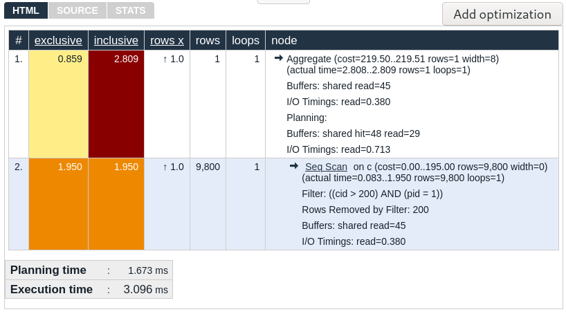
🌐 Since reading a longer execution plan is quite cumbersome, you can use the website https://explain.depesz.com/ to better visualize the query. If you paste the execution plan in the text area and hit “Submit”, you will get output like this:
优化查询的小技巧 #
🌐 Tips for optimizing queries
- 添加索引: 通过在经常用于 WHERE 子句或 JOIN 条件的列上添加索引来提升性能。
- 避免选择未使用的列: 使用 SELECT 只指定你需要的列。
- 更新统计信息: 确保统计信息是最新的,以帮助优化器做出更好的选择。
结论 #
🌐 Conclusion
理解 EXPLAIN 和 EXPLAIN ANALYZE 的输出可以大大提高你编写高效 SQL 查询的能力。定期分析查询性能,并随着数据集的增长和变化进行调整。
🌐 Understanding EXPLAIN and EXPLAIN ANALYZE output can significantly enhance your ability to write efficient SQL queries. Regularly analyze query performance and make adjustments as your dataset grows and changes.
想了解更多信息,你也可以看看:https://aws.amazon.com/blogs/database/how-postgresql-processes-queries-and-how-to-analyze-them/。
🌐 For more insights, you can also check out: https://aws.amazon.com/blogs/database/how-postgresql-processes-queries-and-how-to-analyze-them/.